Split Faced Air-Cooled

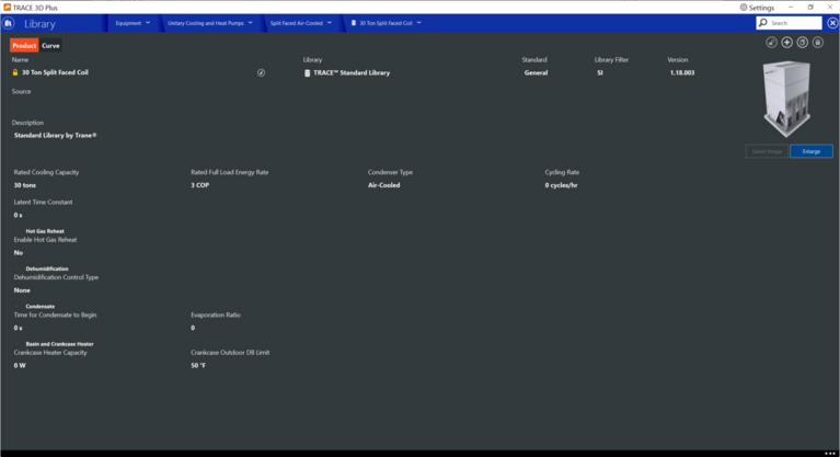
To model a Split Faced Air Cooled Coil in the model first select a DX system type through the Select Systems tab. Go to Configure Systems and navigate to the Properties of the selected system. In the Properties navigate to Components and expand the cooling coil component. Under Type change from Air Cooled to Split Faced Air-cooled and choose the appropriate Split Faced Air Cooled library member.
The Split Faced Air Cooled library member can be used to model DX units with two stages (two sets of cooling coils split horizontally) as well as an enhanced dehumidification mode. The library member curves section defines the overall performance for each stage and mode of operation. Split Faced Air Cooled units can have up to 2 stages of operation for each of the normal cooling mode and enhanced dehumidification mode.
For most cases the Rated Airflow will be the same for all stages and modes of operation associated with the Split Face Air Cooled unit. If there is bypass air specified for the coil the Rated Airflow will include both the bypassed airflow as well as airflow through the active coil.
The Split Faced Air Cooled unit requires entries for the Rated Cooling Capacity, Reference Rated Sensible Heat Ratio, Reference Rated Energy Rate, and the Reference Rated Airflow via the Curve tab. These 4 inputs are used to determine the coil performance at the rating point (air entering cooling coil at 80F DB/67F WB and air entering the condenser at 95F DB/75F WB).
The model requires five curves as follows:
1. The Capacity Curve (function of temperature) is a biquadratic curve with two independent variables: wet-bulb temperature of the air entering the cooling coil, and dry-bulb temperature of the air entering the air-cooled condenser coil (wet-bulb temperature if modeling an evaporative-cooled condenser). The curve is normalized to 1 at 67F indoor wet-bulb temperature and 95F outdoor dry-bulb temperature. The output of this curve is multiplied by the Reference Rated Cooling Capacity to give the total cooling capacity at specific temperature operating conditions (i.e., at temperatures different from the rating point temperatures).
2. The Capacity Airflow Curve (function of flow fraction) is a quadratic or cubic curve with the independent variable being the ratio of the actual air flow rate across the cooling coil to the rated air flow rate (i.e., fraction of full load flow). The curve is normalized to have the value of 1.0 when the actual air flow rate equals the rated air flow rate. The output of this curve is multiplied by the Reference Rated Cooling Capacity and the Capacity Curve (function of temperature) to give the gross total cooling capacity at the specific temperature and air flow conditions at which the coil is operating.
3. The Ambient Relief Curve (function of temperature) is a biquadratic curve with two independent variables: wet-bulb temperature of the air entering the cooling coil, and dry-bulb temperature of the air entering the air-cooled condenser coil (wet-bulb temperature if modeling an evaporative-cooled condenser). The curve is normalized to 1 at 67F indoor wet-bulb temperature and 95F outdoor dry-bulb temperature. The output of this curve is multiplied by the rated Energy Input Ratio (inverse of the rated COP) to give the EIR at specific temperature operating conditions (i.e., at temperatures different from the rating point temperatures).
4. The Power – Airflow Curve (function of flow fraction) is a quadratic or cubic curve with the independent variable being the ratio of the actual air flow rate across the cooling coil to the rated air flow rate (i.e., fraction of full load flow). The curve is normalized to have the value of 1.0 when the actual air flow rate equals the rated air flow rate. The output of this curve is multiplied by the rated EIR (inverse of the rated COP) and the Ambient Relief curve (function of temperature) to give the EIR at the specific temperature and air flow conditions at which the coil is operating.
5. The Part Load Fraction Curve (function of part load ratio) is a quadratic or cubic curve with the independent variable being part load ratio (sensible cooling load / steady-state sensible cooling capacity). The output of this curve is used in combination with the rated EIR and Ambient Relief Curves to give the effective EIR for a given simulation timestep. The part load fraction (PLF) curve accounts for efficiency losses due to compressor cycling. The curve should be normalized to a value of 1.0 when the part-load ratio equals 1.0 (i.e., the compressor(s) run continuously for the simulation timestep).